wVargram: Variogram representation and modeling
wVargram: Variogram representation and modeling
wVargram is the MiraMon tool that represents and models the so-called semivariogram, the spatial pattern describing the correspondence between semivariance and distance. The semivariance (variance * .5) constitutes a measure of the dispersion of the expected values for some variable, and is calculated as the sum of of the squares of the deviations from the mean. The semivariogram (or variogram, as it is often called, as they are basically conceptual equivalents) permits the analysis of the spatial behavior of a property or variable for a particular zone of study, and its modeling constitutes a key element within the process of geostatistical interpolation (kriging).
The essential functionality of this module is to build and analyze the empirical variogram, as well as model it by means of generating the adjusted variogram as a possible sum of the combination and implementation of various of the elemental variograms: nugget, spherical, quadratic, linear, Gaussian and exponential. The variable to model is introduced into the process as a specific field from the database associated with the structured point file (PNT) and the modeled variogram can be saved as an ASCII file in the VAM format.
The variogram's construction consists in two stages organized into two tabs in the wVargram interface.
In the first stage, the properties of the point sample are set, and the geometric and grafic parameters of the empirical Variogram are defined:
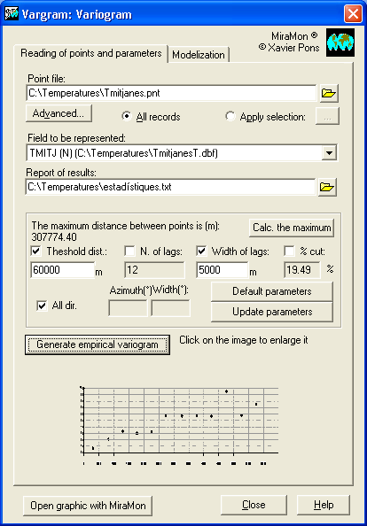
First, the user must define the point file corresponding to the data sample to be analyzed. If necessary, is is possible to carry out a selection from the data, in which case only the selected points will be used in the process. The field from the database containing the variable to be represented and/or modeled must also be chosen.
The user must also specify a file to which will be written: the results report, a text file with information about the origin file, the geometric and graphic parameters and a list of intervals with the names of point pairs belonging to each interval as well as the mean and semivariance assigned to the interval.
The geometric and graphic parameters to define are the following (if required, the maximum distance between points can be requested at any time by using the "Calculate maximum" button):
In the graphic space, multiples of the HRS units can be used, for example
km, if the interval width is adequate.
The distance threshold, number of intervals and interval width are
interrelated such that the distance threshold corresponds to the
number of intervals multiplied by the interval width.
By default, the system processes calculations with 10 intervals and a cut
of 50%, values that by default can be recuperated in any moment by pressing
the corresponding button.
It may also be useful to use the parameter refresh button to see how a
change in one parameter effects the others.
The last step in this first stage (once the adjustable parameters are set and stable) is to Generate the empirical variogram. This draws one point for each interval in a graphic where distances are depicted horizontally and the semivariance of the point pairs assigned to each corresponding interval are depicted vertically. Consulting the alphanumeric point database, the user can obtain the specific values of the mean and semivariance with a far superior precision than that graphically observed. This graphic has three levels of visualization:

In summary, this initial setting of parameters creates, and is one of the main objectives of, the empirical variogram.
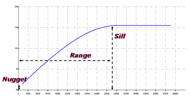
The second stage has the main goal of generating the modeled variogram as well as of determining the corresponding structural parameters of its spatial pattern. In the first step, the user selects the elemental variograms with the appropriate parameters that together will form the composite adjusted variogram. The graphic representation of the parameters that define these elemental variograms is seen in the following figure:
It is advisable to consult a few specialized references at this point in
order to understand some of the details of this structure: two significant
works at the introductory level are:
Oliver, M. A., Webster, R. (1990), "Kriging: a method of
interpolation for geographical information systems". International
Journal of Geographical Information Science, 4:3, 313 - 332
Kitanidis P.K. (1997) Introduction to geostatistics: applications
to hydrogeology. Cambridge University Press.
This second modeling creates the adjusted modelled variogram, and, if considered valid, will be used in the InterPnt module for kriging.
|
|
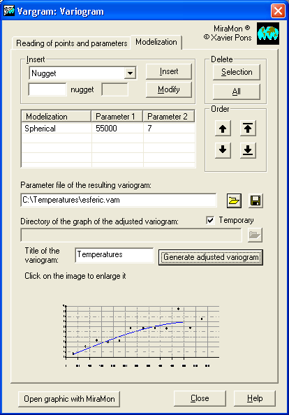
The first part of the Modeling tab corresponds with the construction of the adjusted variogram as the sum of a few implemented elemental variograms: nugget, spherical, quadratic, linear, Gaussian and exponential The resulting variogram parameter file is a VAM file that can be loaded from a file saved to disk, or else it can be generated newly and saved at any time. The program saves it as well by generating the adjusted variogram. 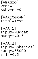 The adjusted variogram's graphic directory can be a temporary directory if the user only wishes to view the graphic, or likewise it can be a specific directory if the user wishes to save it to disk for future use. In the same way, in the points and parameter view tab a preview of the graphic is generated, which can be made larger by clicking on it with the mouse pointer, thereby generating a MiraMon graphic that can be consulted with the button Open graphic in MiraMon: |
|
|
|