-
 CorrGeom: Geometric correction of raster and vector files
Direct access to online help: CorrGeom
Access the application from the menu:
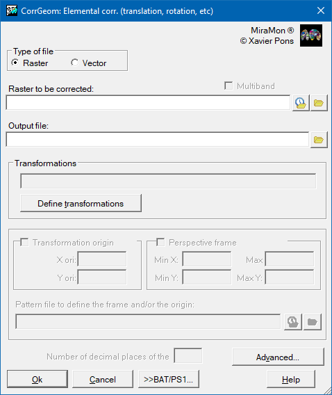
"Tools | Geometry | Elemental corrections (translation, rotation, etc)"
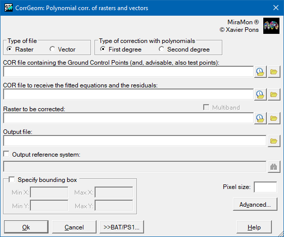
"Tools | Geometry | Polynomial corrections (rasters and vectors)"
"Tools | Geometry | Satellite orthoimage generation"
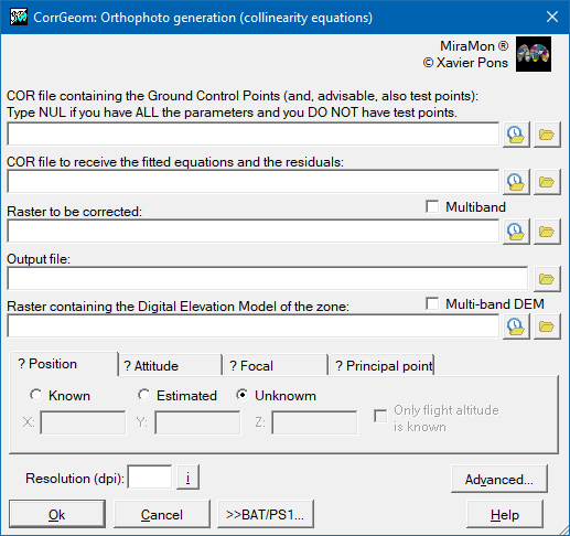
"Tools | Geometry | Orthophoto generation"
Presentation and options
Introduction
Conventional paper maps give us an enormous amount of information which can be incorporated in to a Geographic Information System (GIS). Although more and more maps are now generated digitally there are still many cases in which digital files are not available, either because we are dealing with documents of a certain age, or because they have been created using conventional analogue techniques, or simply because we don't have access to the original digital information.
In these cases, although digitization using a digitizing table may be a possibility it requires a laborious effort and a loss of detail compared to the possibility of scanning the digital document and proceeding to its digitization on the computer screen.
MiraMon allows documents from practically any scanner (in formats BMP, TIFF, JPG, etc) to be transformed to IMG or JPG formats (if they were not already in one of these formats). Once in these formats it is possible to digitize over them the contour lines, roads, land use polygons, etc and convert them in to vector layers. As the scanned documents are still not georeferenced when we digitize directly over them the resultant vector coordinates will be in some arbitrary units (pixels) of the scanning system and not in the map units of the desired georeferenced coordinate system (for example, in meters in the UTM system). Although it is possible to proceed in this way and to georeference the resultant vector document after digitizing using the MiraMon CorrGeom program, it is advisable to georeference the raster first and then to proceed to its digitization . This will also allow map sheets to be scanned separately and then precisely mosaiced together as well as permitting them, once georeferenced, to be displayed with any other available digital vector information layer overlain for reference. Georeferencing of scanned raster files can also be performed using the MiraMon CorrGeom program. So, in summary, there are two alternatives for introducing vector layers into GIS from scanned paper documents using the CorrGeom MiraMon program:
- Scan -> Digitize -> Georeference the vectors
- Scan -> Georeference the raster ->Digitize (RECOMMENDED)
In both cases the recommended method is the first order polynomial fit. In the very unlikely case, given the quality of modern scanners, that the scanned images show quadratic distortions, use the second order polynomial fit.
There exist a number of other interesting sources of information for incorporation in our GIS: such as raster layers like remotely sensed images and aerial photography. These data can be obtained directly in digital format (this is the case for the majority of remotely sensed images) or, alternatively, they may be available in paper or photographic form (the usual case for conventional aerial photography) which can be scanned to convert them into digital images.
Remotely sensed images present a series of geometric distortions produced by the rotation and curvature of the Earth, the irregularities of the platform's orbit, etc. The MiraMon CorrGeom program allows such images to be corrected to remove these distortions using conventional techniques based on first and second order polynomials. In the case of aerial photographs and remotely sensed images with a high level of detail (50m or smaller pixel size) it is advisable to perform corrections taking into account the effect of the relief of the land surface. CorrGeom offers the methods "polynomial fit with heights" for satellite images with small pixels (Landsat TM, SPOT XS and P, IRS LISS, etc) and "collinearity equations fit" for aerial photographs which applies fundamental photogrammetric equations. The images that have been corrected using information about the relief contained in a Digital Elevation Model (DEM) are known as orthoimages (or orthophotos in the case of aerial photos).
The CorrGeom program therefore allows the correction of these distortions (due to the platform's orbit, the relief, etc) and adapts the images to a known cartographic projection system, such as UTM. Once in the appropriate projection system the images can be overlain with other images and vector layers referenced to the same projection system.
Whether correcting raster or vector data it is usual to have a set of ground control points (GCP) which indicate a number of coordinate points in both the uncorrected original reference system and in the final, corrected, reference system. The GCPs can be input with a text editor or digitized as points in MiraMon and converted into GCPs with VECCOR (see below).
In the case of images acquired with a system for which the position and attitude of the sensor are known with precision (GPS+INS) it is possible to do the correction without GCPs.
To increase the statistical reliability of the geometric correction process CorrGeom allows a control points file to contain two subsets of points, one that is used to determine the transformation equations for the fit and the other, which we call the test points, that is used to estimate the error of the fit based on an independent set of points. For both sets of points CorrGeom provides the RMS error in X, Y and globally for each point as well as for the set of control points. Logically, if only one set of points is given then the RMS errors are only given for this set.
If the user wishes to change the projection system, whether of raster or vector datasets, once they have been georeferenced with MiraMon (or if they were imported into MiraMon with georeferences) then the MiraMon program CanviPrj can be used. Do not confuse the functions of CorrGeom that allows non-georeferenced layers to be georeferenced and CanviPrj that changes the projection of layers for which the georeference is already known.
NOTES:
- When we speak of a projection system we are referring to UTM, Lambert, etc, whilst when we speak of a reference system we are referring to, for example, UTM-31N-UB/ICC (ie. the UTM with huso 31, Northern hemisphere, European ED50 datum with the UB/ICC adjusted parameters), or Goode_Homolosine-WGS84 (Goode Homolosine WGS84 with the WGS 1984 datum), etc. (see the help on Geodesia for more information)
- From now on we refer to images and vectors that have been adapted to some reference system using CorrGeom as "corrected".
CorrGeom
The CorrGeom application allows the geometric correction of rasters (IMG and JPG: satellite images aerial photographs, scanned maps...) or vector layers (VEC, PNT, ARC and their derivatives POL and NOD) using a series of n known control points:
- Coordinates in the original reference system ("uncorrected system"), eg. in pixel units, typically with the origin at (0,0) in the bottom left corner in rasters, or eg. in cm in a file coming from the digitization of a vector paper map created on a digitizing tablet and calibrated in centimeters on the map sheet. We will call these units original reference system coordinates: X_SistOri, Y_SistOri.
- Coordinates of the chosen reference system ("corrected" or "map" system, for example UTM-31N). These coordinates are determined manually with the help of map sheets, on the screen with other digital maps, with GPS in the field, etc. We will call these coordinates reference system coordinates : X_SistDest, Y_SistDest [, Z_SistDest].
In addition, the program allows to apply affine transformations (translations, rotations, tilts, scaling and mirrors) and perspective to both rasters and vectors.
All the bands of a multiband raster (typically a 24 bit RGB or a multispectral satellite image) can be geometrically corrected simultaneously by using the /MULTIBANDA parameter or by activating the corresponding button. All the bands will then be corrected in a single operation whilst maintaining a multiband raster as the output. In this case we recommend editing the control points using the band with the highest resolution. If the correction requires the use of a digital elevation model (DEM) and the different bands have different pixel sizes it is possible to use a multiband DEM with as many bands as there are different pixel sizes by activating the parameter /MDE_MULTIBANDA.
The correction can be performed using various methods:
First degree polynomial fit (raster case):
This method does not consider height information (elevation). Typically it is used to correct raster data with little distortion, such as scanned images and maps that were previously corrected (like orthophotos or topographic maps) or satellite images in areas with little marked relief, limited extent, and a relatively large pixel size in relation to the altitude of the satellite. If the objective is to obtain cartography with high geometric quality then the application of these methods to scanned aerial photographs or relatively detailed and extensive satellite images (like SPOT or Landsat-TM) is only appropriate in regions with flat relief.
First degree polynomial fit (vectorial case):
This method does not consider height information (elevation). Typically it is used to correct vector data with little distortion.
Polynomial fit with Z for the columns and first order polynomial without Z for the rows:
With this method of polynomial fit with Z for the columns and first order polynomial without Z for the rows, the fit of the columns is made using a polynomial that simultaneously takes into account X, Y and Z. As for the rows, the fit can be made in three different ways: considering that there is no pitching movement of the sensor during the acquisition of the image, considering that the pitch is constant or considering that the pitch varies linearly. For more details see:
Palà, V., Pons, X. (1995) Incorporation of relief into geometric corrections based on polynomials. Photogrammetric Engineering & Remote Sensing, 61(7):935-944.
Polynomial fit with Z for columns with constant pitch and 1st degree polynomial with Z for rows:
In this case, analogous to the previous one but with constant pitch and 1st degree polynomial with Z for the rows, the fit of the columns is made using a polynomial that simultaneously takes into account X, Y and Z. As for the rows, the fit can be made in three different ways: considering that there is no pitching movement of the sensor during the acquisition of the image, considering that the pitch is constant or considering that the pitch varies linearly. For more details see:
Palà, V., Pons, X. (1995) Incorporation of relief into geometric corrections based on polynomials. Photogrammetric Engineering & Remote Sensing, 61(7):935-944.
Polynomial fit with Z for columns with variable pitch and 1st degree polynomial with Z for rows:
With this method, similar to the previous one with variable pitch, the fit of the columns is made using a polynomial that simultaneously takes into account X, Y and Z. As for the rows, the fit can be made in three different ways: considering that there is no pitching movement of the sensor during the acquisition of the image, considering that the pitch is constant or considering that the pitch varies linearly. For more details see:
Palà, V., Pons, X. (1995) Incorporation of relief into geometric corrections based on polynomials. Photogrammetric Engineering & Remote Sensing, 61(7):935-944.
Collinearity equations fit:
The parameters used in the collinearity equations are: position (Xc, Yc, Zc) and attitude (omega, fi, kappa) of the camera or sensor, the camera focal length (f) and the coordinates of the principal point (x_pp, y_pp) of the image. The user may decide which of these parameters to estimate by fitting and which are set. For those which are to be estimated it is useful to give some approximate values which will help the program converge more rapidly. In some cases, if the initial parameter is completely unknown or the approximation is very poor, the algorithm may not converge or unsatisfactory solutions may be produced. If all the parameters are known and set then the transformation is performed without using control points and using the test points just to evaluate the error of the fit. These are the initial values of the flight parameters in the first iteration:- Roll: omega = 0
- Pitch: fi = 0
- Yaw: kappa = Various values are tried and the one that gives the smallest RMS in the first iterations is used.
- Xc = Average of the X coordinates of the control points (in the reference system).
- Yc = Average of the Y coordinates of the control points (in the reference system).
- ZZc = Average Zc + flight altitude, approx. 2000-3000 m
When the principal point (x_pp, y_pp) has to be fit the program takes as initial values:- x_pp = Average of the x coordinates (in original units) of the control points or the middle of the raster.
- y_pp = Average of the y coordinates (in original units) of the control points or the middle of the raster
However, sometimes these averages can be quite distant from the real principal point and in these cases the program may not converge (eg if only a fragment from the edge of an aerial photograph is scanned). The program allows the user to change the value for another estimated by eye at the intersection of the lines joining the fiducial points. Remember to use always the same measurement system, consistent with the original reference units.
For fitting the focal length it is necessary to choose some initial value close to the real value, typically between 15 and 35 mm for digital cameras and between 50 and 250 mm for analogical cameras.
In addition it is necessary to know the number of points per inch (ppp, ppi or dpi) of the scanned image (1 inch = 25.4 mm). For analogue photos common values are between 400 and 200 dpi. For digital photos refer to the manufacturer's technical specifications (for example the AA497-AMDC 28.0 camera with 2024 columns x 2041 rows and a sensor size of 18x18 mm gives a resolution of 2811-2835 dpi).
Geometric Transformations (raster case):
These types of transformations follow a different philosophy from the previous ones: instead of adjusting the transformation using control points, we want to specify the transformation parameters ourselves because we know them a priori. For instance, we may have scanned a document rotated 90º to fit better into the scanner once rotated; in this case, it will be easier to indicate that we want to apply a 90º rotation to return it to its original position and view it in a "natural" way (perhaps before placing control points for fine-tuning the geometry). A second example would be having a dataset where the horizontal reference system units are in km, and we want to convert them to meters, which requires applying a scaling factor of 1000.
The types of operations offered are translations, scalings, shears, rotations, perspectives, and mirrors. For affine transformations (all except perspective), a transformation origin can be specified, and for perspective, an envelope over which to act can be specified. The possibility of choosing this is provided so that if we want to modify a vector layer over an already modified raster, we can use the raster's envelope to perfectly overlay the transformed vector layer onto the modified raster.
It is possible to perform a sequence of transformations and/or a perspective one after the other on a raster or vector, with the sole restriction that only one perspective can be used.
Geometric Transformations (vectorial case):
These types of transformations follow a different philosophy from the previous ones: instead of adjusting the transformation using control points, we want to specify the transformation parameters ourselves because we know them a priori. An example would be having an old vector dataset from software that stored coordinates with single precision (such as PC-Arc/Info) and, for this reason, truncated the most significant digit when it was constant for the entire layer (for example, in Catalonia in UTM-31N, it was common to omit the 4 from the Y coordinate, so a coordinate like 4619254.734 was written as 619254.734, maintaining decimetric precision); in this case, we can recover the original coordinates by specifying a translation transformation of magnitude 4000000. Finally, a third example would be having a dataset where the horizontal reference system units are in km, and we want to convert them to meters, which requires applying a scaling factor of 1000. The types of operations offered are translations, scalings, shears, rotations, perspectives, and mirrors. For affine transformations (all except perspective), a transformation origin can be specified, and for perspective, an envelope over which to act can be specified. The possibility of choosing this is provided so that if we want to modify a vector layer over an already modified raster, we can use the raster's envelope to perfectly overlay the transformed vector layer onto the modified raster. It is possible to perform a sequence of transformations and/or a perspective one after the other on a raster or vector, with the sole restriction that only one perspective can be used.
Adjustment based on reference points:
In this case, the geometric correction is made from two rasters that, when paired, provide the origin position of each pixel of the destination image (therefore, they typically have the same dimensions as this one) and together they form, therefore, a mesh of reference.
The procedure is based on the following: For each pixel center of the desired output raster (rectified, corrected, georeferenced, depending on what the coordinates are used for), the program searches for the values of this position in the reference rasters (one for the axis of the X and the other by the Y axis), which ends up providing the specific pixel in the image to be corrected that is closest to the coordinates of the reference rasters. The value in the source raster will be assigned to this output raster pixel when the rescan method is nearest neighbor, or it will be interpolated from neighbors in the other available rescan methods. By default, the output file will have the same envelope, pixel side, and reference system as the XY reference rasters.
Note on the COR file format:
COR files contain the ground control points and, optionally, test points, in the following format:
 Number_of_points [Comments]
 X_OriSyst1 Y_OriSyst1 X_DestSyst1 Y_DestSyst1 [Z_DestSyst1] [Comments1]
     :          :          :           :            :            :
- Z coordinate Z_DestSyst1 are not required in the first two options of the program.
- Test points (optional) will be written, with the same format, below this sequence. The user must write at the start of the relevant block the number of test points.
- The file may end with comments of indefinite length, which the program does not preserve and which are replaced by the results of the adjustment.
- The "Original System" coordinates must be Cartesian, i.e., the coordinates must increase positively rightwards in x and upwards in y. The coordinate 0,0 can be either at any point of the original file or even outside it.
This format can be generated with a text editor or from a file of points digitized over the original file. This file can be easily transformed to COR format using the VECCOR program.
For raster images and for program options that do not require input of either the resolution or the bounding rectangle of the output file, these parameters are taken from the DEM documentation file. The maximum envelope values of the output file are adapted as a function of the value of the output resolution (res) using the following expression:
    Xmax = Xmin + res * rounding_by_ceiling (Xmax-Xmin/res)
    Ymax = Ymin + res * rounding_by_ceiling (Ymax-Ymin/res)
The number of rows and columns of the output image can be determined from:
    Ncolumns = rounding_by_ceiling (Xmin-Xmin/res)
    Nrows = rounding_by_ceiling (Ymax-Ymax/res)
The background or NoData value will be written in the corrected file when the uncorrected file has no data for the output cells in that position.The user may choose the NoData value or allow the program to set this. By default it will be the same as the input, if this exists or, if there are no NoData values in the original data, the default is 255 for byte/byte-RELimages or the smallest allowable negative value for all other formats. If theimage to be corrected is byte/byte-REL and has no defined NoData value, and if when it is corrected NoData values are generated then by default the original valid values that in the output correspond to NoData will be saturated. In 24-bit images reduced to 8-bit images with an optimized palette this can lead to an incorrect visualization so consequently an option is given for the program to reclassify these values to the closest colour index so that the display remains practically unchanged.
The program supports digital elevation models of type BYTE, INTEGER (short) and REAL, compressed and uncompressed.

Dialog box of the application
Graphic examples
First degree polynomial corrections
 |
Detail of the placement of a control point at the UTM-06N coordinate (453000,7194000),
North America datum 1983, on a 1:25000 USGS topographic map in Alaska Fairbanks.
The careful placement of a point at each of the 4 ends of the map allows to obtain, georeferenced,
the cartographic document with an RMS that has an adjustment of 28 cm with the scanned document
(in reality, since the map is at a scale of 1:25000 the real RMS on the ground must be about 5 m). |
Polynomial corrections with Z
 |
 |
| Adjustment points located on a SPOT image ((c) SPOT-Image) |
General aspect of the correction of the previous SPOT image on
an ICGC orthophoto (areas with NoData are shown transparent). |
 |
 |
| Detail of the correction of the previous SPOT image compared to an image from the ICGC. The reference grid has a side of 1 km. |
Corrections with collinearity equations
 |
 |
| Adjustment (A) and test (T) points located in a frame from the Cartographic and Geological Institute of Catalonia (ICGC). |
Detail of the correction of the previous frame, converted into an orthophoto (left) compared with an orthophoto from the ICGC (right) in order to appreciate the very good geometric fit achieved. Each pixel in the image corresponds to 50 cm. |
Syntax examples
For raster images:
CorrGeom 1 MAP MA2 LANDSAT.img  LND 0 450000 480500 4724500 4750000 30 /NODATA=0
CorrGeom 2 MAP NUL LANDSAT.img  LND 1  X  X  X   X  30
CorrGeom 4 MAP MA2 LANDSAT.img  ORTOLND 1 MDE30
CorrGeom 6 MAP MA2 FOTOSCAN.img ORTOFOT 1 MDE05 400 20 153 1475 1512
For vector files
CorrGeom 1 MUNIPC_1 MUNIPC_2 MUNI_1.pnt MUNI_COR
CorrGeom 2 MUNIPC_1 NUL  MUNI_1.arc MUNI_COR
CorrGeom 1 MUNIPC_1 MUNIPC_2 MUNI_1.vec MUNI_COR 0
For geometric transformations (afines and perspective):
6.5 units translation in positive vertical direction:
CorrGeom 7 LANDSAT.img LND 0 T 0 6.5
7 units translation in negative horizontal direction:
CorrGeom 7 LANDSAT.img LND 0 T -7 0
45 degrees clockwise rotation:
CorrGeom 7 LANDSAT.img LND 0 R 45
45 degrees anticlockwise rotation:
CorrGeom 7 LANDSAT.img LND 0 R -45
Scaling ratio 2 (in both directions: vertical and horizontal) plus 90º clockwise rotation:
CorrGeom 7 LANDSAT.img LND 0 E 2 2 R 90
Slight inclination in horizontal right direction:
CorrGeom 7 LANDSAT.img LND 0 I x 0.1
50% inclination in horizontal left direction:
CorrGeom 7 LANDSAT.img LND 0 I x -1
Perspective of points in a raster which has a perspective (of 0.5).
Supose that the envelope of the raster is (XMIN, YMIN)=(0,10), (XMAX, YMAX)=(4500, 6000)
CorrGeom 7 MUNI_1.pnt MUNI_COR P 0.5 /XMIN=0 /XMAX=4500 /YMIN=10 /YMAX=6000 Notice that if we don't apply the optative parameters, these points won't adapt to the modified raster.
Rotation of points in a raster which has been also rotated (45º).
Supose that the envelope of the raster is (XMIN, YMIN)=(0,10), (XMAX, YMAX)=(4500, 6000)
CorrGeom 7 MUNI_1.pnt MUNI_COR R 45 /XORI=0 /YORI=10
Notice that if we don't apply the optative parameters, these points won't adapt to the modified raster.
Scaling from cm to m and after translate 4000000 m in Y's.
The arguments of affine transformations are transformed for the program itself, so, we can think this operation as:
Scaling from cm to m. Translate 400000000 cms in Y's.
CorrGeom 7 Fitxer.arc Fitxer_sor.arc E 100 100 T 0 400000000
For adjustment based on reference points:
CorrGeom 8 Fitx_in.img Fitx_out.img Fitx_X.img Fitx_Y.img 0 x x x x
CorrGeom 8 Fitx_multi_in.img Directori Fitx_X.img Fitx_Y.img 0 x x x x /MULTIBANDA /PREFIX=apr_
Syntax
Syntax:
- CorrGeom 1 CorFile ErrCorFile InRasFile OutRasFile resampling xMin xMax yMin yMax res [/NODATA] [/PALETA] [/MULTIBANDA] [/PREFIX] [/SIST_DEST]
- CorrGeom 1 CorFile ErrCorFile InVecFile OutVecFile [/N_DECIMALS] [/SIST_DEST]
- CorrGeom 2 CorFile ErrCorFile InRasFile OutRasFile resampling xMin xMax yMin yMax res [/NODATA] [/PALETA] [/MULTIBANDA] [/PREFIX] [/SIST_DEST]
- CorrGeom 2 CorFile ErrCorFile InVecFile OutVecFile [/N_DECIMALS] [/SIST_DEST]
- CorrGeom 3 CorFile ErrCorFile InRasFile OutRasFile resampling DEM [/NODATA] [/PALETA] [/MULTIBANDA] [/PREFIX] [/MDE_MULTIBANDA]
- CorrGeom 4 CorFile ErrCorFile InRasFile OutRasFile resampling DEM [/NODATA] [/PALETA] [/MULTIBANDA] [/PREFIX] [/MDE_MULTIBANDA]
- CorrGeom 5 CorFile ErrCorFile InRasFile OutRasFile resampling DEM [/NODATA] [/PALETA] [/MULTIBANDA] [/PREFIX] [/MDE_MULTIBANDA]
- CorrGeom 6 CorFile ErrCorFile InRasFile OutRasFile resampling DEM Resolution Iterations PositOpt AttitOpt FocalOpt PrincPtOpt [/XCAM] [/YCAM] [/ZCAM] [/WCAM] [/FCAM] [/KCAM] [/FOCAL] [/ANALOG] [/DIGITAL] [/XPP] [/YPP] [/PMPCONTROL] [/PMRASTER] [/NODATA] [/PALETA] [/MULTIBANDA] [/PREFIX] [/MDE_MULTIBANDA]
- CorrGeom 7 InRasFile OutRasFile resampling [T] [Tx] [Ty] [E] [Ex] [Ey] [I] [Id] [Ir] [R] [g] [P] [Pr] [M] [Md] [/NODATA] [/PALETA] [/MULTIBANDA] [/PREFIX] [/MDE_MULTIBANDA] [/YORI] [/XMAX] [/XORI] [/YMIN] [/XMIN] [/YMAX]
- CorrGeom 7 InVecFile OutVecFile [T] [Tx] [Ty] [E] [Ex] [Ey] [I] [Id] [Ir] [R] [g] [P] [Pr] [M] [Md] [/YMIN] [/XMIN] [/YMAX] [/YORI] [/XMAX] [/XORI] [/N_DECIMALS]
- CorrGeom 8 InRasFile OutRasFile XCoorFile YCoorFile resampling XMinTrim XMaxTrim YMinTrim YMaxTrim [/MULTIBANDA] [/PREFIX] [/NODATA] [/PALETA] [/SIST_DEST]
Options:
- 1:
First degree polynomial fit (raster case).
- 1:
First degree polynomial fit (vector case).
- 2:
Second degree polynomial fit (raster case).
- 2:
Second degree polynomial fit (vector case).
- 3:
Polynomial fit with Z for the columns and first order polynomial without Z for the rows.
- 4:
As for 3 but with a constant pitch and Z for the rows.
- 5:
As for 3 but with a variable pitch and Z for the rows.
- 6:
Collinearity equations fit.
- 7:
Geometric Transformations (raster case).
- 7:
Geometric Transformations (vector case).
- 8:
Adjustment based on reference points.
Parameters:
- CorFile
(Control -
Input parameter): Name of the file containing ground control points in COR format.
- ErrCorFile
(Control error -
Output parameter): Name of the COR file that will contain the equations and the errors of the fit and the test points. The user may select NUL for automatic corrections where this file is not wanted.
- InRasFile
(Image file -
Input parameter): The raster file to be corrected (with extension).
- OutRasFile
(Output raster file -
Output parameter): Name of the output corrected file (without extension) or the name of the directory of the corrected files in the case of multiband images.
- resampling
(Resampling type -
Input parameter): Criterion for deciding the output pixel value (resampling type):
- 0: Nearest neighbor (thematic maps; conserve the original radiometric signal).
- 1: Bilinear interpolation (images for photointerpretations; DEMs).
- 2: I Bicubic interpolation (as 1; smoothed results but slower).
- xMin
(X minimum -
Input parameter): The X minimum output raster bounding coordinates. Type 'x x x x' if you want the program to calculate them (the entire input raster will be corrected).
- xMax
(Maximum X -
Input parameter): The X maximum output raster bounding coordinates. Type 'x x x x' if you want the program to calculate them (the entire input raster will be corrected).
- yMin
(Y minimum -
Input parameter): The Y minimum output raster bounding coordinates. Type 'x x x x' if you want the program to calculate them (the entire input raster will be corrected).
- yMax
(Y maximum -
Input parameter): The Y maximum output raster bounding coordinates. Type 'x x x x' if you want the program to calculate them (the entire input raster will be corrected).
- res
(Output resolution -
Input parameter): Resolution of the output image in map units.
- InVecFile
(Vectorial file to be corrected -
Input parameter): The vectorial file to be corrected (with extension).
- OutVecFile
(Output vector file -
Output parameter): Name of the output corrected file (without extension).
- DEM
(Digital Elevation Model -
Input parameter): Raster file with the DEM of the region.
- Resolution
(Resolution -
Input parameter): For scanned images or digital photos, the resolution in dots per inch (dpi).
- Iterations
(Iterations -
Input parameter): Maximum number of iterations when using the collinearity equations (sugg. 20).
- PositOpt
(Position Options -
Input parameter): Option (position) that define whether the parameters used in the collinearity equations are set and known (3), estimated (2) or unknown (0). The value (1) is for the special case where only the flight altitude is estimated but not the X, Y position of the plane.
- AttitOpt
(Attitude options -
Input parameter): Options (attitude) that define whether the parameters used in the collinearity equations are set and known (3), estimated (2) or unknown (0).
- FocalOpt
(Focal option -
Input parameter): Option (focal) that define whether the parameters used in the collinearity equations are set and known (3), estimated (2) or unknown (0).
- PrincPtOpt
(Principal point options -
Input parameter): Option (principal point) that defines whether the parameters used in the collinearity equations are set and known (3), estimated (2) or unknown (0).
- T
(Translation -
Input parameter): Indicate translation
- Tx
(X value -
Input parameter): X value of the translation.
- Ty
(Y Value -
Input parameter): Y Value of the translation
- E
(Scaling -
Input parameter): Indicate scaling geometric transformation.
- Ex
(X value -
Input parameter): X value
- Ey
(Y value -
Input parameter): Y value
- I
(Inclination -
Input parameter): Indicate an inclination geometric transformation.
- Id
(Inclination axis -
Input parameter): Indicate the axis the inclination.
- Ir
(Indicate inclination reason. -
Input parameter): Inclination reason.
- R
(Rotation -
Input parameter): Indicate Rotation.
- g
(Degrees -
Input parameter): Degrees
- P
(Perspective -
Input parameter): Indicate perspective.
- Pr
(Perspective reason -
Input parameter): Indicate perspective reason.
- M
(Mirror -
Input parameter): Indicate mirror.
- Md
(Mirror direction -
Input parameter): Indicate mirror direction. If we want to make a mirror with respect to the horizontal axis we must use the value 'x' (or 'X'). If we want to make a mirror with respect to the vertical axis we must use the value 'y' (or 'Y').
- XCoorFile
(X coordinate file -
Input parameter): It is the name of the raster file (with extension) with X coordinates where the value is searched for in the source file.
- YCoorFile
(Y coordinate file -
Input parameter): It is the name of the raster file (with extension) with Y coordinates where the value is searched for in the source file.
- XMinTrim
(X Minimum to trim -
Input parameter): The minimum X coordinate of the scope of the destination file is indicated. If 'x' is indicated, the minimum X of the X and Y coordinate file will be chosen.
- XMaxTrim
(X Maximum to trim -
Input parameter): The maximum X coordinate of the scope of the destination file is indicated. If 'x' is indicated, the minimum X of the X and Y coordinate file will be chosen.
- YMinTrim
(Y Minimum to trim -
Input parameter): The minimum Y coordinate of the scope of the destination file is indicated. If 'x' is indicated, the minimum X of the X and Y coordinate file will be chosen.
- YMaxTrim
(X Maximum to trim -
Input parameter): The maximum Y coordinate of the scope of the destination file is indicated. If 'x' is indicated, the minimum X of the X and Y coordinate file will be chosen.
Modifiers:
/XCAM=
(X camera)
X coordinate of the camera or sensor in the output reference system. They may be known positions or estimated values. If only /ZCAM is given then this indicates that only the plane altitude is estimated. (Input parameter) /YCAM=
(Y camera)
Y coordinate of the camera or sensor in the output reference system. They may be known positions or estimated values. If only /ZCAM is given then this indicates that only the plane altitude is estimated. (Input parameter) /ZCAM=
(Z camera)
Z coordinate of the camera or sensor in the output reference system. They may be known positions or estimated values. If only /ZCAM is given then this indicates that only the plane altitude is estimated. (Input parameter) /WCAM=
(Omega)
Indicate in degrees the omega attitude angle of the sensor, whether set or estimated. (Input parameter) /FCAM=
(Phi)
Indicate in degrees the "phi" attitude angle of the sensor, whether set or estimated. (Input parameter) /KCAM=
(Kappa)
Indicate in degrees the "kappa" attitude angle of the sensor, whether set or estimated. (Input parameter) /FOCAL=
(Focal)
Indicates in millimeters the known or estimated focal length of the camera. (Input parameter) /ANALOG
(Analogic camera)
If the focal length of the camera is unknown, knowing whether it is digital or analog (this case) helps to take an initial value that converges more quickly to the adjusted value. (Input parameter) /DIGITAL
(Digital camera)
If the focal length of the camera is unknown it can be useful to know whether the camera is digital or analogue when selecting an initial value that is more likely to produce a rapid convergence to the fit value. (Input parameter) /XPP=
(XPP)
X coordinate or approximate initial values of the principal point in the original coordinates. (Input parameter) /YPP=
(YPP)
Y coordinate or approximate initial values of the principal point in the original coordinates. (Input parameter) /PMPCONTROL=
(Estimated control points)
If the location of the principal point is unknown, then the initial values can be estimated as the average of either the control points or the central point of the raster to be corrected. (Input parameter) /PMRASTER=
(Average point raster)
Average raster point (Input parameter) /MDE_MULTIBANDA (Multiband Digital Elevation Model) For simultaneously correcting multiband rasters having different pixel sizes and for which there are DEMs for each cell size. (Input parameter) /YMIN= (Minimum Y of the area to apply transformation.) Minimum Y coordinate of the area in which you want to apply the transformation. It is only useful when a perspective is applied because in transformations without perspective /XORI, /YORI is used. (Input parameter) /XMIN= (Minimum X of the area to apply transformation.) Minimum X coordinate of the area in which you want to apply the transformation. It is only useful when a perspective is applied because in transformations without perspective /XORI, /YORI is used. (Input parameter) /YMAX= (Maximum Y of the area to apply transformation.) Maximum Y coordinate of the area in which you want to apply the transformation. It is only useful when a perspective is applied because in transformations without perspective /XORI, /YORI is used. (Input parameter) /YORI= (Transformation origin on the Y axis) Indicates the origin on the Y axis of the transformation if there is any. (Input parameter) /XMAX= (Maximum X of the area to apply transformation.) Maximum X coordinate of the area in which you want to apply the transformation. It is only useful when a perspective is applied because in transformations without perspective /XORI, /YORI is used. (Input parameter) /XORI= (Transformation origin on the X axis) Indicates the origin on the X axis of the transformation if there is any. (Input parameter) /N_DECIMALS= (Number decimals) Number of the coordinates of the vector output. Only for VEC files. (Input parameter) /MULTIBANDA (MULTIBANDA) To simultaneously correct multiband raster images and to generate corresponding corrected bands. (Input parameter) /PREFIX= (Prefix) For multiband images, the prefix to add to the original files when creating the corrected files. By default the prefix is c_. (Input parameter) /NODATA= (NoData) NoData value for the corrected image. If the user is completely sure that there will be no NoData (after checking the geometry of the transformation, the extent, the range of the DEM...) then it is possible to give the value "NONE". (Input parameter) /PALETA= (Paleta) Palette (p25, pal, p65) or symbol table (dbf) that determines which colour index is closest to the NoData index for the corrected image. (Input parameter) /SIST_DEST= (Output reference system) Identifier of the projection system of the output file. (Input parameter)