| Presentation and options | Dialog boxes of the application |
| Graphic examples | Syntax |
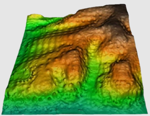
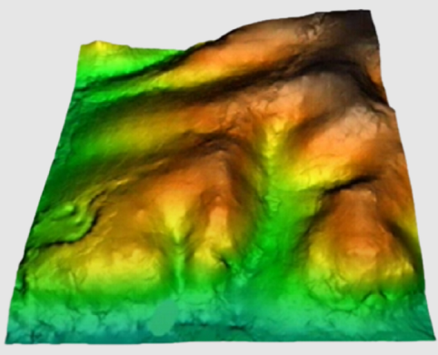
As for most of the calculation procedures, interpolation between points can give widely different results according to the choice of options in the application. The chosen method, the threshold distance, the weighting applied, the use of exclusion masks, etc., can help to improve results enormously. Knowledge of the data to be processed and the use of trial runs with varying parameters can be a great help in order to select how best to use these parameters. Furthermore, if possible, it is useful to keep back a set of randomly distributed and independent points in order to carry out a quantitative evaluation (test) of the results.
In quantile calculations, such as the median, it is possible to indicate, with the modifier /MEDIANA_EMPAT=, the type of tiebreaker to be used for its calculation when the position of the quantile is between two values of the series. For more information, see general syntax.
In the current version there are five possible interpolation methods: the inverse distance and the spline function, trend surfaces, kriging and neighborhood statistics.
For the inverse distance method, the interpolation of each point (cell) is carried out by assigning weights to the values of the sample points in inverse proportion to the distance that separates each sample point from the center of the pixel. This distance can be calculated as a Euclidean distance, or using the simplified (Manhattan/Taxi Cab) distance. For more information, please consult https://en.wikipedia.org/wiki/Inverse_distance_weighting.

For the spline method a regular, continuous and derivable function, or set of functions if the area is divided into different regions, is determined which best adapts to the sample points without loosing its property of continuity. For more information on the analytical expression of this function consult:

Regarding the method of generating trend surfaces, it is about adjusting a polynomial function with respect to the X, Y of degree 1, 2 or 3 that will result in a smooth, continuous and derivable surface resulting from the adjustment. This adjustment is done by least squares and will allow to determine the coefficients of each term of the polynomial.

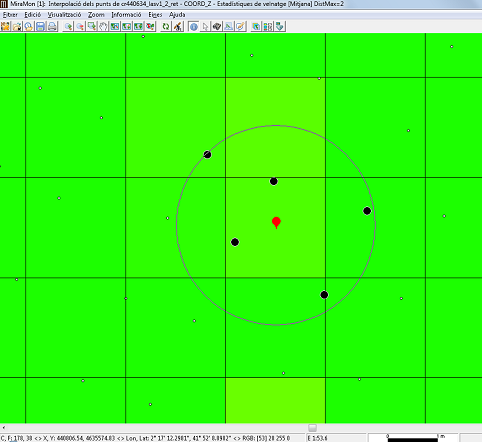
With the neighborhood statistics method, the designated statistic (mean, median, maximum, minimum, range, standard deviation, mean absolute deviation around the median or number of occurrences, percentile) is assigned to each cell, calculated considering all the points that are within a circle defined by a radius, or within a square defined by one side, located in the center of each cell that is to be interpolated. Unlike other methods of InterPNT, and in particular of the method that makes the interpolation by weighting a user-defined power of inverse distance but also limits this calculation to a certain distance radius (maximum distance), in the neighborhood statistics mode once all the points present within the indicated scope (circular or square) are selected, no weighting is done but the requested calculation is made directly, which can be a measure of the centrality of the different values (average or median), of dispersion of these values (maximum, minimum, range, standard deviation, mean absolute deviation around the median) or, simply, a count of the number of available values (number of occurrences).
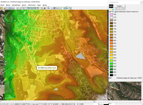
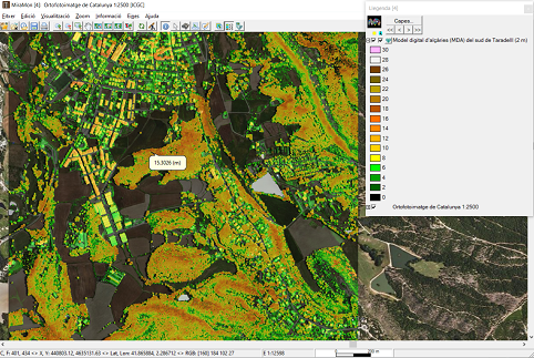
This is a typical method for processing lidar data, and particularly for the production of Digital Surface Models (DSM) or Digital Height Models (DHM). In these two applications, the highest elevation obtained by the lidar in the raster cell area to be obtained is usually taken. This area can be the area of the cell if the point density is high enough in relation to the size of the cell, or somewhat larger (for example a radius 1.5 times the side of the cell); please consult the specific options below for more details.
If the point density is very high, instead of the maximum, a 90 percentile, etc. can be requested, which reduces the probability of adopting as a real surface some sensor artifact such as the detection of birds flying at that moment. With other statistics, such as dispersion statistics, interesting data on the vertical structure of vegetation masses can be obtained. Finally, by choosing the minimum as statistics, combined with the selection of points corresponding to unique returns (information available in one of the fields of the attribute table) and high return intensities (data also available in another field), and with very large scan radii (several times the cell side to be obtained), a Digital Elevation Model (DEM) can be obtained. If a DEM is already available, or it has been calculated with lidar data as just described, a DHM can be obtained (the altimetric data of vegetation or human constructions are measured from the ground and not above sea level); in this case the most practical thing is, before running InterPNT, to run the application CombiCap in the form DEM+PNT-->PNT and with the statistical field transfer mode using bilinear interpolation, where the second PNT will obtain the elevations at each point; An empty numeric field is then generated, typically with 2 or 3 decimal places, so that, using CalcImg, it can be filled with the point height (calculated as the subtraction between the altitude obtained from the lidar and the elevation obtained from CombiCap). This height is the one that is submitted to InterPNT to obtain the MDH.
General procedure
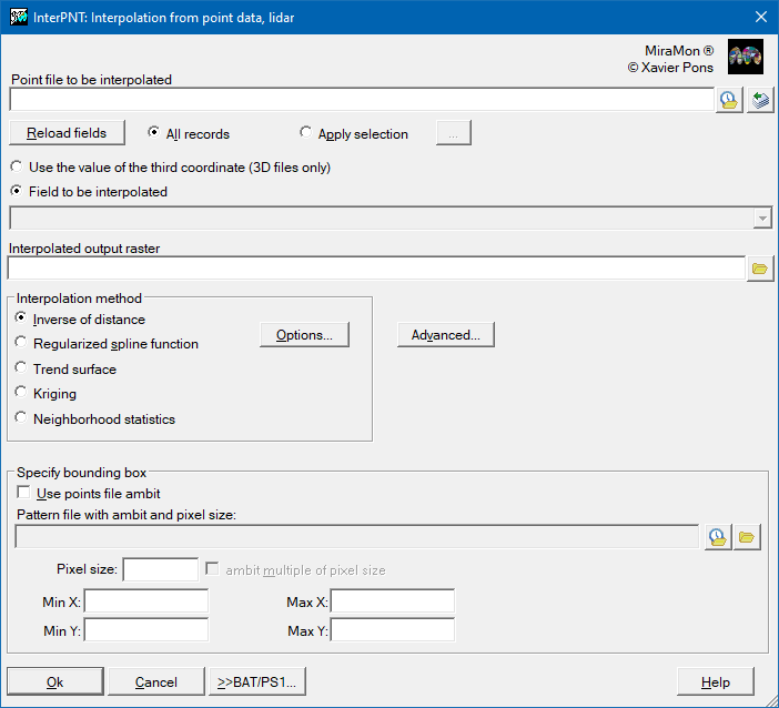
First of all, it is necessary to choose whether to use the value of the third coordinate (in the case of 3D files) or to select a field to interpolate the database associated with the points file. In the case of choosing a database field, you must select a numeric field. Although the values of this field can be integers, the interpolator will treat these data as double precision real values in all internal calculations and generate an output raster with real precision.
The selection of records is the first filter that chooses which records, in the points database, will be considered in the interpolation. The default option is 'All records', but often the quality and speed of the interpolation can be improved if those records that we do not want to influence the result are excluded. The choice of records is made by constructing a logical sentence based on any combination of the fields in the database associated with the points file. Notice that the fields involved in the selection do not necessarily have to be used in the interpolation. For example, in a file containing atmospheric emissions one field could indicate the district where each industry is located and, if we wish to interpolate values of a certain pollutant, we could choose to interpolate only the values for a particular district. We recommend using the option that can be opened from the 'Apply selection' option in order to construct the logical sentence, based on a selection of fields, operators, values, links and orders of priority using the buttons and the corresponding pull-down menus. In the section on the 'Syntax' of the command line, the elements of this sentence are detailed. This works in a similar way to queries on MiraMon attributes.
The output file will be an uncompressed real value raster (except when exclusion masks are defined, in which case it will be compressed and real). This raster will have a predefined background, or NoData, value in those cells for which no value could be calculated because at that location it was not possible to satisfy the criteria of the 'Advanced Options', either because the point was inside an exclusion mask or because it did not have a minimum of points within the maximum allowable distance.
It is necessary to define the extent and cell size for the output raster by either giving the corner co-ordinates or by adjusting the extent to the area covered by the file with the points. It should be noted that the speed of the process is very sensitive to these values. A small cell size in a large interpolation area without any defined mask will give very precise values (that vary smoothly as a function of distance), but the number of calculations will be very large and the execution time will be long.
Inverse distance options
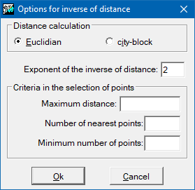
It is necessary to define, firstly, how to calculate distances; whether as a Euclidean distance, or as a 'Manhattan' distance (see previous section for the definitions of both distances). The value assigned to each cell is a weighted average of the values of the points under consideration. The weight given to each point is proportional to the inverse of an exponential power of the distance between the point and the center of the pixel. The default value of this exponential power is 2, but this parameter can be changed in the way that the user considers most appropriate. The bigger the value, the more weight given to the points nearest to the pixel and the less weight given to more distant points.
The maximum distance is a commonly used parameter. It establishes the region of influence of each point as a circle centered on the point and with a radius equal to the maximum distance. Thus, for each cell we have a distance beyond which the original points play no part in the interpolation process. It is advisable to always use this parameter since, apart from intuitively making sense in the interpolation process, it also allows the execution time to be reduced considerably.
Another interesting criterion is to define a maximum number of points to use in the interpolation. Evidently these will always be the 'n' points nearest to the center of the pixel. The repeated ranking process needed to apply this criterion slows down the calculation considerably, but the use of this criterion assures that only the 'n' nearest points are taken into account. To make sure that the calculation is done with a sufficient sample it is also possible to define a minimum number of points for the interpolation at each cell. If this minimum is not reached the cell's value will be NoData.
Spline options
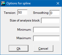
Interpolation by splines can be very sensitive to the configuration parameters, depending on the sample points. The tension parameter modulates the smoothing of the function; its default value is 40 and excessively high or low tensions can lead to unexpected effects. The flattening parameter adjusts the noise of the sample, the default value is 0 which implies that the function passes exactly through the sample points (exact interpolation). The analysis block size parameter limits the fit by dividing the area into analysis blocks and restricting the solution of the spline functions to this region. This parameter speeds up the process considerably. It is recommended when there are many points available, but it can produce unwanted discontinuities if the block size is too small (analysis window too local).
The spline interpolation method works optimally for samples without excessive disturbances. However, when points are close to each other and have abrupt variations for the variable to be interpolated this method may result in values which are well outside the expected range. In this case, it is recommended to increase the tension value and to choose the complementary option that enforces the output results to be between a maximum and a minimum. Thus, it will be necessary to define the modifies /MIN_VAL i /MAX_VAL.
If the analysis block size is not defined, a single solution is found for the whole region covered by the raster (the window is the same as the raster extent). If the size is small the area is divided into many independent regions.
Options for trend surfaces
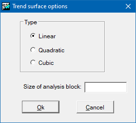
The main parameter of this option is the degree that determines the order of the polynomial to adjust. In the current version it is possible to generate first-degree or linear, second-degree or quadratic and third-degree or cubic surfaces.
In the same way that for spline, it is possible to generate different solutions, not strictly continuous, by dividing the global scope into more local sub-regions. These sub-regions are defined by the side of the analysis block parameter.
Opciones para el kriging
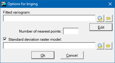
The kriging interpolation method is based on the principles of geostatistics. In order to apply it, it is necessary to have previously generated an adjusted variogram file (with the extension "vam"). This file can be generated with the Vargram application, in which help instructions can be found about how to model the spatial pattern of the variable to be analyzed that gives rise to the variogram that will be applied for interpolation with this method. In the advanced options of InterPNT, it is also possible to limit the number of points closest to each cell that participate in its resulting value, as well as obtain an auxiliary raster of the quality of the estimate, where the standard deviations for each cell will be stored. More information about kriging can be found at https://en.wikipedia.org/wiki/Kriging.
Options for neighborhood statistics
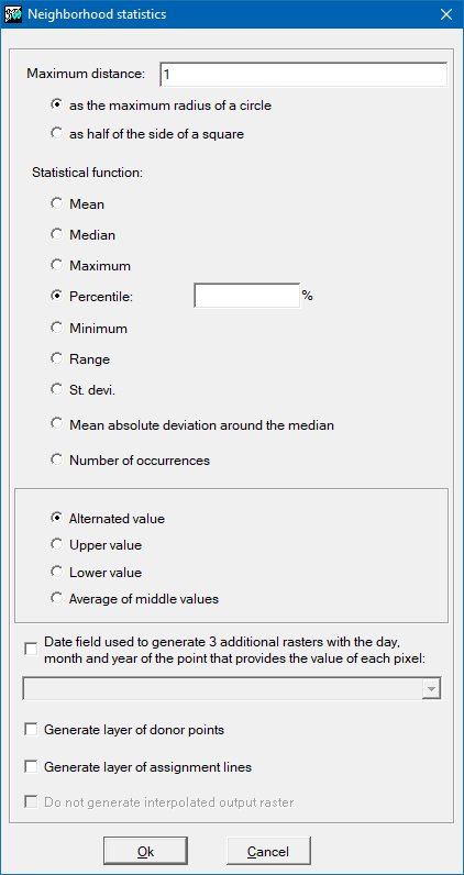
Two parameters must be defined: the statistical function to be used, and the maximum distance at which a point is considered to be part of the set of points that provide the values for the calculation of the statistics to be transferred to the cell of the raster output.
The statistical functions available are the average, the median, the maximum, the minimum, the rank, the standard deviation, the mean absolute deviation around the median and the number of occurrences.
For the maximum distance there are two possible options: maximum distance as maximum radius of a circle, and maximum distance as half of the side of a square. This last option is typically used when it is desired that the lidar points with which the statistical value will be calculated are strictly located within the cell; note that, since the data is half of the square, if a 2-meter-side raster is desired, the distance to be indicated for the maximum distance will be 1 meter. When the calculated statistic value comes from a single point, as in the case of the minimum and maximum, it is possible to generate additional layers (with the same name as the output layer and an appropriate suffix): On one hand, if the lidar data provides, in separate fields, the day, month, and year of the capture of each point, it is possible to generate 3 additional rasters that will contain the day, month, and year of the point providing the value for each pixel. On the other hand, for educational and research purposes, it is possible to generate additional layers containing only the donor points or that connect the donor points with lines to the center of the cell that receives the value.
Advanced options
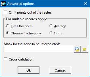
The advanced options allow finer adjustment of the parameters of some of the global interpolation procedures.
For the case where there is more than one record associated with a chosen point (e.g., where there are various measurements at different times at the same water source), we can choose how to interpolate the value from this point: The options are a) ignore this point as a multiple record (as though it did not form part of the selection); b) select the value of the first record that satisfies the selection conditions; c) take the average of the records; d) take the sum of the values.
Another possibility is to select points so that those that fall outside the area of the raster are ignored. This option is not recommended if the values near the borders of the raster are important.
Finally, we can also decide whether for some regions inside the area of the raster, it is necessary or not to know the results of the interpolation. Using a file that acts as an exclusion mask and so determining which areas are useful and which are not, we can accelerate considerably the calculation process, and we obtain more coherent results for pointless exclusion zones; for example, if we are interpolating elevations from spot heights we can exclude all sea areas. This mask may be a raster in which the regions to be excluded will be those with NoData values in the cells. The mask may also be a structured or unstructured polygon vector file. In this case the area to be excluded will be, by default, the universal polygon, otherwise the mask will include those polygons with attributes equal to or different from some explicitly defined value. For structured vectors it is also necessary to specify which field from the attribute table will define the mask.
 |
|||
 |
 |
 |
 |
 |
|||
 |
|||
| InterPNT dialog boxes | |||
